Example of using PyImfit to Estimate B/T Uncertainties
This is a Jupyter notebook demonstrating how to use PyImfit and bootstrap resampling to estimate uncertainties for derived quantities of fits, such as \(B/T\) values.
If you are seeing this as part of the readthedocs.org HTML documentation, you can retrieve the original .ipynb file here.
Introduction
PyImfit will estimate uncertainties for individual model parameters from a fit (if you use the default Levenberg-Marquardt minimizer) – e.g., position \(X0,Y0\), position-angles, ellipticities, scale lengths, etc.. You can also estimate parameter uncertainties via bootstrap resampling, or by using an external Markov-Chain Monte Carlo algorithm (see here for an example of the latter).
Sometimes, you might also want to have some estimate of derived values based on a model, such as the total luminosity or the bulge/total (\(B/T\)) value (assuming you have some idea of which component in your model is the “bulge”). How do you determine the uncertainties for such quantities? This notebook shows a simple example of how one might do that, using PyImfit’s bootstrap-resampling option.
The basic idea is to generate a set of model-parameter vectors via,
e.g., bootstrap resampling (or from an MCMC chain). You then compute the
resulting derived quantity from those parameter values. In this
particular case, we use the pyimfit.Imfit object containing the
model to compute “bulge” and total flux values for each parameter
vector, and then take the ratio to get \(B/T\) values. By doing this
for all the parameter vectors, you end up with a distribution for the
derived quantity.
Preliminaries
Some initial setup for nice-looking plots:
%pylab inline

matplotlib.rcParams['figure.figsize'] = (8,6)
matplotlib.rcParams['xtick.labelsize'] = 16
matplotlib.rcParams['ytick.labelsize'] = 16
matplotlib.rcParams['axes.labelsize'] = 20
Populating the interactive namespace from numpy and matplotlib
Create an image-fitting model using PyImfit
Load the pymfit package; also load numpy and astropy.io.fits (so we can read FITS files):
import numpy as np
import pyimfit
from astropy.io import fits
Load the data image (here, an SDSS \(r\)-band image cutout of VCC 1512) and corresponding mask:
imageFile = "./pyimfit_bootstrap_BtoT_files/vcc1512rss_cutout.fits"
image_vcc1512 = fits.getdata(imageFile)
maskFile = "./pyimfit_bootstrap_BtoT_files/vcc1512rss_mask_cutout.fits"
mask_vcc1512 = fits.getdata(maskFile)
Create a ModelDescription instance based on an imfit configuration file (which specifies a Sersic + Exponential model):
configFile = "./pyimfit_bootstrap_BtoT_files/config_imfit_vcc1512.dat"
model_desc = pyimfit.ModelDescription.load(configFile)
print(model_desc)
ORIGINAL_SKY    120.020408
GAIN    4.725000
READNOISE   4.300000
X0      60.0
Y0      73.0
FUNCTION Sersic
PA      155.0       90.0,180.0
ell     0.2     0.0,0.5
n       2.05        0.0,4.0
I_e     120.0       0.0,10000.0
r_e     4.5     0.0,20.0

FUNCTION Exponential
PA      140.0       90.0,180.0
ell     0.28        0.0,0.8
I_0     70.0        0.0,10000.0
h       20.0        0.0,200.0
Create an Imfit instance containing the model, and add the image and mask data. Note that we are not doing PSF convolution, in order to save time (this is not meant to be a particular accurate model).
imfit_fitter = pyimfit.Imfit(model_desc)
imfit_fitter.loadData(image_vcc1512, mask=mask_vcc1512)
Fit the model to the data (using the default Levenberg-Marquardt solver) and extract the best-fitting parameter values:
results = imfit_fitter.doFit(getSummary=True)
print(results)
           aic: 21156.824446201397
           bic: 21242.642276390998
  fitConverged: True
       fitStat: 21134.809840392267
fitStatReduced: 1.169219398118625
         nIter: 10
     paramErrs: array([0.01518161, 0.0167467 , 1.88166351, 0.00733777, 0.01613089,
      1.9553319 , 0.05896027, 0.65080573, 0.00529781, 1.11196358,
      0.18740197])
        params: array([6.04336387e+01, 7.32059007e+01, 1.61799952e+02, 1.18947666e-01,
      9.56352657e-01, 1.21814611e+02, 4.86558532e+00, 1.38986928e+02,
      2.73912311e-01, 8.13853830e+01, 2.08521933e+01])
    solverName: 'LM'
p_bestfit = results.params

print("Best-fitting parameter values:")
for i in range(len(p_bestfit) - 1):
    print("{0:g}".format(p_bestfit[i]), end=", ")
print("{0:g}\n".format(p_bestfit[-1]))
Best-fitting parameter values:
60.4336, 73.2059, 161.801, 0.118946, 0.956308, 121.821, 4.86538, 138.987, 0.273911, 81.389, 20.8517
Run bootstrap-resampling to generate a set of parameter values (array of best-fit parameter vectors)
OK, now we’re going to do some bootstrap resampling to build up a set of several hundred alternate “best-fit” parameter values.
Note that you coul also generate a set of parameter vectors using MCMC; we’re doing bootstrap resampling mainly because it’s faster.
Run 500 iterations of bootstrap resamplng. More would be better; this is just to save time (takes about 1 minute on a 2017 MacBook Pro).
bootstrap_params_array = imfit_fitter.runBootstrap(500)
bootstrap_params_array.shape
(500, 11)
Use these parameter vectors to calculate range of B/T values
We define a function to calculate the \(B/T\) value, given a parameter vector (for this model it’s simple, but you might have a more complicated model where the first component isn’t necessarily the “bulge”).
def GetBtoT( fitter, params ):
    """
    Get the B/T value for a model parameter vector (where "bulge" is the first component
    in the model)

    Parameters
    ----------
    fitter : instance of PyImfit's Imfit class
        The Imfit instance containing the model and data to be fit
    params : 1D sequence of float
        The parameter vector corresponding to the model

    Returns
    -------
    B/T : float
    """
    total_flux, component_fluxes = fitter.getModelFluxes(params)
    # here, we assume the first component in the model is the "bulge"
    return component_fluxes[0] / total_flux
The \(B/T\) value for the best-fit model:
GetBtoT(imfit_fitter, p_bestfit)
0.1557485598370547
Now calculate the \(B/T\) values for the bootstrap-generated set of parameter vectors:
n_param_vectors = params_array.shape[0]
b2t_values = [GetBtoT(imfit_fitter, bootstrap_params_array[i]) for i in range(n_param_vectors)]
b2t_values = np.array(b2t_values)
And now we can analyze the vector of B/T values …
For example:
np.mean(b2t_values)
0.15852423639167879
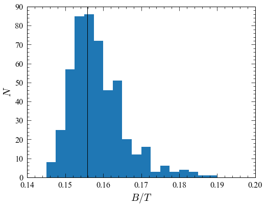
A histogram of the \(B/T\) values (vertical line = best-fit value):
hist(b2t_values, bins=np.arange(0.14,0.2,0.0025));xlabel(r"$B/T$");ylabel(r"$N$")
axvline(GetBtoT(imfit_fitter, p_bestfit), color='k')
<matplotlib.lines.Line2D at 0x12c671a10>
png